General

StrainTool allows the estimation of Strain Tensor parameters, on the earth's crust, given a list of data point, aka points on the earth along with their tectonic velocities.

StrainTool has three basic components:

• A python package, named pystrain
• The main executable, named StrainTensor.py
• A list of shell scripts to plot results from StrainTensor.py

pystrain Package

pystrain is a package written in python, defining a variety of functions, classes, etc to enable the computation of strain tensors.

When installing this package, all of its modules will be available to the user. It is the core part of the project and should be installed before the main program (StrainTensor.py) can be used.

The package is found under StrainTool/pystrain

StrainTensor.py

This is the main program, i.e the program that the user will run to produce strain tensor results. It is heavily dependant on the pystrain package (so any change there will affect StrainTensor.py's behaviour

This program does not need installation; it is just a pyrhon script. The user may only need to change priviledges to make it executable

StrainTensor.py is located at StrainTool/bin

Plot Tools

By 'Plot Tools', we mean an array of shell (Bash) scripts that can be used to plot StrainTensor.py results. These scripts actualy use GMT to perform the plotting. The scripts are an efficient, ready-to-use

It is by no means mandatory to use these scripts to plot the results; users can use their own tools and/or scripts to do so. Actualy, this is a totaly independent part of the Project and can be skipped alltogether.

These scripts, are found under StrainTool/plot

Installation

Prerequisites

To install the Project, you will need:

• python; the installation has been tested under Versions 2.7 and 3.6 and both work fine.
• NumPy; NumPy is the fundamental package for scientific computing with Python.
• SciPy; SciPy is a Python-based ecosystem of open-source software for mathematics, science, and engineering. Actualy, we are only using the SciPy.linalg and SciPy.spatial modules.

Installation Procedure

To install the Project, you actualy only need to install the pystrain package. What this means, is that python will see that the package modules are build and extracted to a suitable folder on your local system (something like /usr/lib/python2.7/site-packages/ on a UNIX-like system). After this step, you will be able to make use of the modules in the package, both for running StrainTool.py and for any new program you may wish to code. StrainTensor.py and Plot Tools are programs, so you do not have to "install" them.

To install pystrain, do the following:

1. go to the directory the package is located, i.e. StrainTool/pystrain
2. the package comes with a setup.py script, so you only need to run it (as root/administrator):

   $> python setup.py install

$> python -c "import pystrain"

Installation tests

The following scenarios have been tested to validatethe installation procedure

Example

To validate that the installation has succeded, you can run a "test case" scenario. Under the folder data/, you will find a file named CNRS_midas.vel. This ascii file, contains velocity and coordinate information for a large list of GPS/GNSS stations around the globe. We will use it to perform a test run of StrainTensor.py.

Go to the bin/ folder and execute the command:

$> ./StrainTensor.py -i ../data/CNRS_midas.vel -r 18.75/30.25/32.75/42.25 --x-grid-step=0.5 --y-grid-step=0.5 --dmin=1 --dmax=500 --dstep=1 --Wt=24 -c -g 

Under data/ you will find the "reference" output files for checking, named strain_info.dat.ref and station_info.dat.ref. Verify that the files you have just created (placed under bin/) contain the same results as the "reference" files (this can be very easily performed using the diff command).

Plot example files and compare

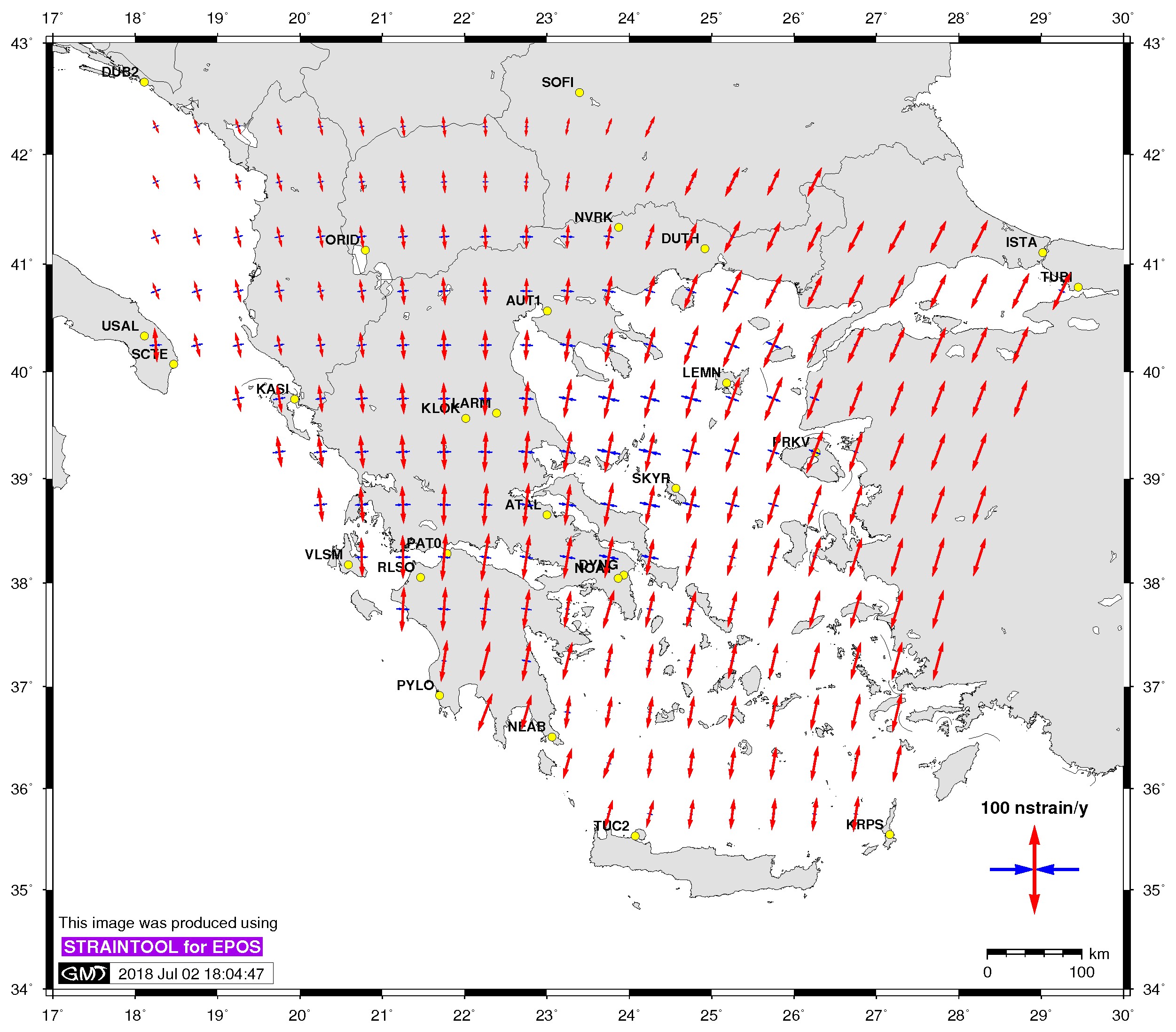
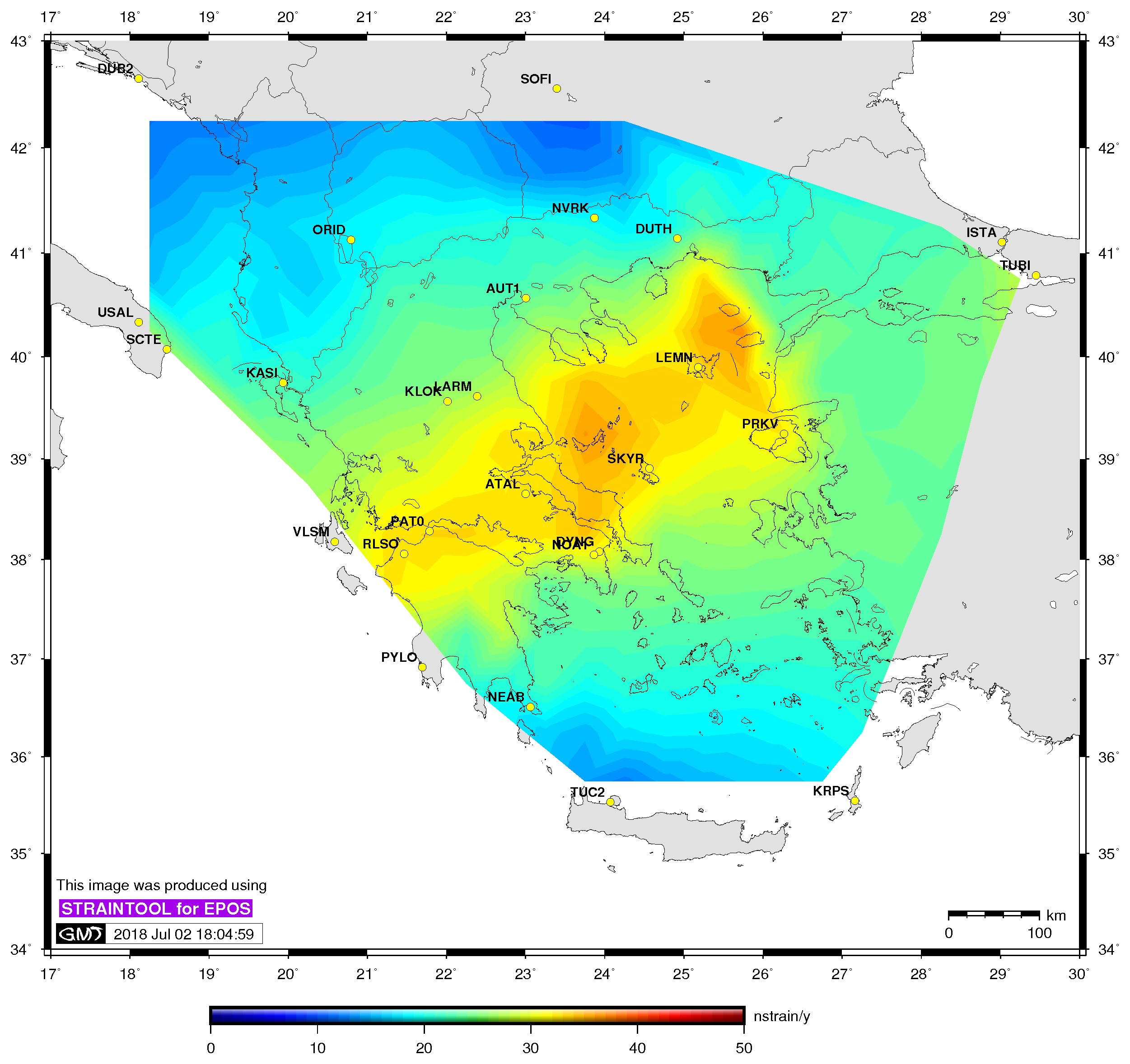
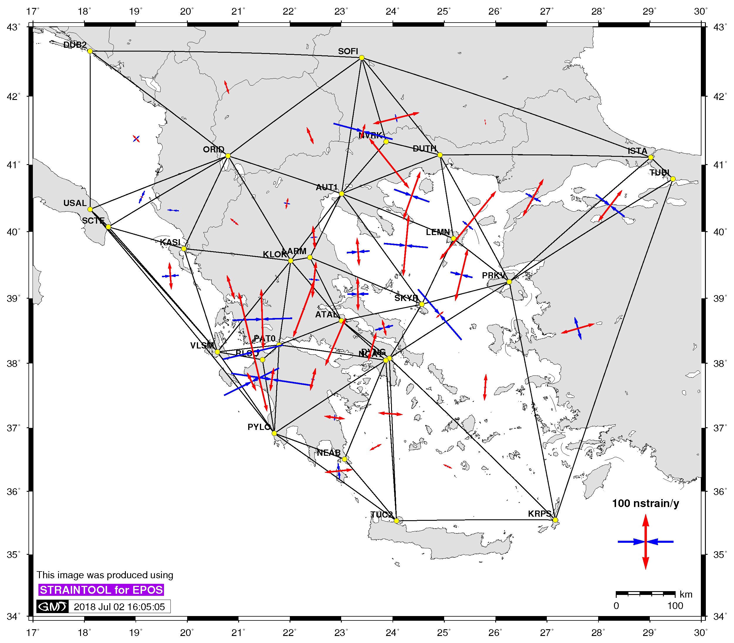
Principal axis	Shear strain	Delaunay triangles
$> ./gmtstrainplot.sh -jpg -str strain_info.dat -psta -l -o output_str	$> ./gmtstrainplot.sh -jpg -gtot strain_info.dat -psta -l -o output_gtot	$> ./gmtstrainplot.sh -jpg -str strain_info.dat -psta -l -o output_str -deltr

How to use StrainTensor.py

StrainTensor.py computes strain tensor parameters on a selected region. The program comes with an extended help message, that can be displayed via the -h or --help switch (aka

$> ./StrainTensor.py [...] --help

Basic Usage

To use the program, the only mandatory switch is the -i or --input-file, which specifies the input file to be used. All other options will automaticaly assume default values (see Options for a detailed list). Basic usage is described below:

usage: StrainTensor.py [-h] -i INPUT_FILE [--x-grid-step X_GRID_STEP]
                       [--y-grid-step Y_GRID_STEP] [-m METHOD] [-r REGION]
                       [-c] [-b] [--max-beta-angle MAX_BETA_ANGLE]
                       [-t WEIGHTING_FUNCTION] [--Wt Wt] [--dmin D_MIN]
                       [--dmax D_MAX] [--dstep D_STEP] [--d-param D_PARAMETER]
                       [-g] [--verbose] [--multicore] [-v]

Options

The whole list of available options, is:

optional arguments:
          -h, --help            show this help message and exit
  -i INPUT_FILE, --input-file INPUT_FILE
                        The input file. This must be an ascii file containing the columns: 'station-name longtitude latitude Ve Vn SigmaVe SigmaVn Sne time-span'. Longtitude and latitude must be given in decimal degrees; velocities (in east and north components) in mm/yr. Columns should be seperated by whitespaces. Note that at his point the last two columns (aka Sne and time-span) are not used, so they could have random values.
  --x-grid-step X_GRID_STEP
                        The x-axis grid step size in degrees. This option is only relevant if the program computes more than one strain tensors. Default is 0.5(deg).
  --y-grid-step Y_GRID_STEP
                        The y-axis grid step size in degrees. This option is only relevant if the program computes more than one strain tensors. Default is 0.5(deg)
  -m METHOD, --method METHOD
                        Choose a method for strain estimation. If 'shen' is passed in, the estimation will follow the algorithm described in Shen et al, 2015, using a weighted least squares approach. If 'veis' is passed in, then the region is going to be split into delaneuy triangles and a strain estimated in each barycenter. Default is 'shen'.
  -r REGION, --region REGION
                        Specify a region; any station (in the input file) falling outside will be ommited. The region should be given as a rectangle, specifying min/max values in longtitude and latitude (using decimal degrees). E.g. "[...] --region=21.0/23.5/36.0/38.5 [...]"
  -c, --cut-excess-stations
                        This option is only considered if the '-r' option is set. If this this option is enabled, then any station (from the input file) outside the region limit (passed in via the '-r' option) is not considered in the strain estimation.
  -b, --barycenter      Only estimate one strain tensor, at the region's barycentre.
  --max-beta-angle MAX_BETA_ANGLE
                        Only relevant for '--mehod=shen'. Before estimating a tensor, the angles between consecutive points are computed. If the max angle is larger than max_beta_angle (in degrees), then the point is ommited (aka no tensor is computed). This option is used to exclude points from the computation tha only have limited geometric coverage (e.g. the edges of the grid). Default is 180 deg.
  -t WEIGHTING_FUNCTION, --weighting-function WEIGHTING_FUNCTION
                        Only relevant for '--mehod=shen'. Choose between a 'gaussian' or a 'quadratic' spatial weighting function. Default is 'gaussian'.
  --Wt Wt               Only relevant for '--mehod=shen' and if 'd-param' is not passed in. Let W=Σ_i*G_i, the total reweighting coefficients of the data, and let Wt be the threshold of W. For a given Wt, the smoothing constant D is determined by Wd=Wt . It should be noted that W is a function of the interpolation coordinate, therefore for the same Wt assigned, D varies spatially based on the in situ data strength; that is, the denser the local data array is, the smaller is D, and vice versa. Default is Wt=24.
  --dmin D_MIN          Only relevant for '--mehod=shen' and if 'd-param' is not passed in. This is the lower limit for searching for an optimal d-param value. Unit is km. Default is dmin=1km.
  --dmax D_MAX          Only relevant for '--mehod=shen' and if 'd-param' is not passed in. This is the upper limit for searching for an optimal d-param value. Unit is km. Default is dmax=500km.
  --dstep D_STEP        Only relevant for '--mehod=shen' and if 'd-param' is not passed in. This is the step size for searching for an optimal d-param value. Unit is km. Default is dstep=2km.
  --d-param D_PARAMETER
                        Only relevant for '--mehod=shen'. This is the 'D' parameter for computing the spatial weights. If this option is used, then the parameters: dmin, dmax, dstep and Wt are not used.
  -g, --generate-statistics
                        Only relevant when '--mehod=shen' and '--barycenter' is not set. This option will create an output file, named 'strain_stats.dat', where estimation info and statistics will be written.
  --verbose             Run in verbose mode (show debugging messages)
  --multicore           Run in multithreading mode (default: False)
  -v                    Display version and exit.

For example, the command we used on the Example section:

$> ./StrainTensor.py -i ../data/CNRS_midas.vel -r 18.75/30.25/32.75/42.25 --x-grid-step=0.5 --y-grid-step=0.5 --dmin=1 --dmax=500 --dstep=1 --Wt=24 -c

Input Files

To perform the computations, StrainTensor.py needs an input file, that holds input data. Usually, this implies a list of GPS/GNSS stations with their ellipsoidal coordinates (aka longtitude and latitude) and their respective tectonic velocities (usually estimated using position time-series) allong with the corresponding standard deviation values. The format of these files, should follow the convention:

        station-name  longtitude   latitude   Ve     Vn    SigmaVe  SigmaVn  Sne  time-span 
         string           deg.        deg.   mm/yr  mm/yr   mm/yr    mm/yr    /   dec. years

There are no strict formating rules on how the individual elements should be printed (i.e. how many fields, decimal places, etc). The only condition is that fields are seperated by whitespace(s). To see an example of a valid input file, you can check data/CNRS_midas.vel.

Output Files

Results of StrainTensor.py are recorded in the following three files:

• strain_info.dat This file includes strain tensor parameters, principal axis, rotational rates, dilatation etc.
  The columns of the file are structured as below:

Latitude Longtitude vx+dvx  vy+dvy   w+dw     exx+dexx    exy+dexy    eyy+deyy   emax+demax  emin+demin   shr+dshr  azi+dazi  dilat+ddilat   sec.inv+dsec.inv 
   deg       deg     mm/yr   mm/yr  deg/Myr   nstrain/yr  nstrain/yr  nstrain/yr  nstrain/yr  nstrain/yr  nstrain/yr    deg.    nstrain/yr    nstrain/yr

• station_info.dat Station's data used for the calculation of strain tensor are written at this file. Format is:

Code    Longtitude Latitude  Ve   Vn   dVe  dVn 
string      deg       deg          mm/yr

• strain_stats.dat This file is only created if the --generate-statistics switch is on. The generated file will hold various information on the system, the command and options used, and statistics of the computation. This file can help users get a quick overview of the program's run.

How to use Plot Tools

Plotting scripts are placed under plot/ directory. They are:

• gmtstrainplot.sh,
• gmtstatsplot.sh, and
• plotall.sh

        pth2inptf=../data/  # set default folder for input files (strain_info.dat, station_info.dat)
	west, east, south, north, projscale, frame, sclength: set region parameters
        STRSC=0.01 : set principal axis plot scale
        ROTSC=.7 : set rotational rates plot scale
        

Basic Plots & Background :
     -r | --region : region to plot (default Greece)
         usage: -r west east south north projscale frame

PLot station and velocitiess:
    -psta [:=stations] plot only stations from input file
    -vhor (station_file)[:= horizontal velocities]
    -vsc [:=velocity scale] change valocity scale default 0.05

Plot strain tensor parameters:
     -str (strain file)[:= strains] Plot strain rates 
     -rot (strain file)[:= rots] Plot rotational rates 
     -gtot(strain file)[:=shear strain] plot total shear strain rate contours
     -gtotaxes (strain file) dextral and sinistral max shear strain rates
     -dil (strainfile)[:= dilatation] Plot dilatation and principal axes
     -secinv (strain file) [:=2nd invariand] Plot second invariand
     -strsc [:=strain scale]
     -rotsc [:=rotational scales]
  *for -gtot | -dil | -secinv use +grd to plot gridded data
        ex:-gtot+grd 


Other options:
     -o | --output : name of output files
     -l | --labels : plot labels
     -mt | --map_title "title" : title map default none, use quotes
     -jpg : convert eps file to jpg
     -h | --help : help menu
        

For example, to plot the principal axis fo strain rates for the example case above you can use the following command:

$>./gmtstrainplot.sh -jpg -str strain_info.dat -psta -l
        

Basic Plots & Background :
     -r | --region : region to plot (default Greece)
         usage: -r west east south north projscale frame

Plot Stations and triangles:
     -psta [:=stations] plot only stations from input file
     -deltr [:= delaunay triangles] plot delaunay triangles

Plot Statistics:
     -stats (input file) set input file
     --stats-stations : plot used stations
     --stats-doptimal : plot optimal distance (D)
     --stats-sigma : plot sigma 

Other options:
     -o | --output : name of output files
     -l | --labels : plot labels
     -leg : plot legends
     -mt | --map_title  : title map default none use quotes
     -jpg : convert eps file to jpg
     -h | --help : help menu
        

For example, to plot the stations used per cell grid for the example case above you can use the following command:

$> ./gmtstatsplot.sh -jpg -stats strain_stats.dat --stats-stations -leg -o output_stats-stations
        

   - no switch produce default output names
   -p | --prefix : add prefix work id to output file
   -s | --suffix : add suffix work id to output file
   -h | --help: help panel
        

For example:

$> ./plotall.sh -p test -s test2
        

Background and Algorithms

Given a set of stations (aka point on earth's surface) with their corresponding east and north velocities, we can estimate (or compute) strain tensor parameters, by solving for the system $$ \begin{bmatrix} V_{x,S_1} \\ V_{y,S_1} \\ V_{x,S_2} \\ V_{y,S_2} \\ \cdots \\ V_{x,S_n} \\ V_{y,S_n} \\ \end{bmatrix} = \begin{bmatrix} 1 & 0 & \Delta_{y_1} & \Delta_{x_1} & \Delta_{y_1} & 0 \\ 0 & 1 & -\Delta_{x_1} & 0 & \Delta_{x_1} & \Delta_{y_1} \\ 1 & 0 & \Delta_{y_2} & \Delta_{x_2} & \Delta_{y_2} & 0 \\ 0 & 1 & -\Delta_{x_2} & 0 & \Delta_{x_2} & \Delta_{y_2} \\ \cdots & \cdots & \cdots & \cdots & \cdots & \cdots \\ 1 & 0 & \Delta_{y_n} & \Delta_{x_n} & \Delta_{y_n} & 0 \\ 0 & 1 & -\Delta_{x_n} & 0 & \Delta_{x_n} & \Delta_{y_n} \\ \end{bmatrix} \begin{bmatrix} U_{x} \\ U_{y} \\ \omega \\ \tau_{x} \\ \tau_{xy} \\ \tau_{y} \\ \end{bmatrix} $$ at any given location \(R\); \(\Delta_{x_i}\) and \(\Delta_{y_i}\) are the displacement components between station \(i\) and the point \(R\). A minimum of 3 stations is required to compute the parameters; if more than 3 stations are used, then the parameters are estimated (here, using a least squares approach).

Covariance Matrix

Assuming that we have variance information for the station velocities (and a Gaussian distribution), we can add the covariance matrix \(C\) of the velocity data in the system. In the simplest case, \(C\) is a diagonal matrix, with the velocity component standard deviations as its elements, $$ C = {\sigma_{0}}^2 \begin{bmatrix} (1/\sigma_{V_{x,S_{1}}})^2 & 0 & 0 & \cdots & 0 \\ 0 & (1/\sigma_{V_{y,S_{1}}})^2 & 0 & \cdots & 0 \\ 0 & 0 & (1/\sigma_{V_{x,S_{2}}})^2 & \cdots & 0 \\ \vdots & \vdots & \vdots & \ddots & \vdots \\ 0 & 0 & 0 & \cdots & (1/\sigma_{V_{y,S_{n}}})^2 \\ \end{bmatrix} $$

Shen et al, 2015, propose a more elaborate approach, reconstructing the covariance matrix by multiplying a weighting function to each of its diagonal terms. The weighting function \(G_i = L_i \cdot Z_i\), in which \(L_i\) and \(Z_i\) are functions of distance and spatial coverage dependent, respectively. The final covariance matrix becomes then, \(C = C \cdot G^{-1}\) or, since its diagonal, \(C_i = C_i \cdot {G_i}^{-1}\)

Shen et al, 2015

The following paragraphs, describe the estimation process when using shen method (i.e. --method=shen) as the algorithm of choice.

In coarse lines, when choosing the shen method, the program will 'girddify' the region of choise and estimate one strain tensor at the centre of each cell. The region of choise can be given via the --region switch, using minimum and maximum longtitude and latitude as decimal degrees, using '/' as delimeter. E.g. [...] --region=21.0/23.5/36.0/38.5 [...]. If the region is not specified, then the maximum and minimum longtitude values will be extracted from the list of input stations, aka the region will be defined to include all stations within the input file.

The user can specify the grid step size, both in x and y components, via the --x-grid-step and --y-grid-step switches respectively. The step sizes should be given in decimal degrees and if not set, have a default value of \(0.5 deg.\)

The program will try to estimate strain tensor parameters at the centre of each cell. The algorithm depends on a number of options that the user can define via the command line arguments. Using a spatial smoothing coefficient \(D\), either defined by the user (--d-param) or found by the program (see Finding the optimal smoothing parameter \(D\)), the covariance matrix will be formed, using distance-dependent weighting \(L_i\), spatial weighting \(Z_i\) and the data variance information \(C_i\). The final covariance matrix, will be \(C \cdot G^{-1}\) where \(G_i = L_i \cdot Z_i\).

Strain tensor parameters will be estimated using a (weighted) least squares approach; Six fundamental parameters are solved for and in a next step values of interest are computed (see Strain Tensor Parameters). Computed values are written to the output file strain_info.dat (see Output Files).

Distance-dependent Weighting

For distance dependent weighting \(L_i\), we can use two formulas, $$L_i = \exp(-{\Delta}R_i^{2} / D^{2})$$ or $$L_i = 1/(1 + {\Delta}R_i^{2} / D^{2})$$ n which a spatial smoothing parameter \(D\) is introduced (see Finding the optimal smoothing parameter). According to Shen et al, 2015,

Both functions allow reduced weight of the data as distance increases. The difference between the two is that the Gaussian function reduces the weight at a faster pace with distance \(\Delta R_i\) than that of the quadratic function. Depending on the data quality, the Gaussian function can offer a relatively finer resolution of the interpolation result if the data are clean and smooth. On the other hand, if the data are somewhat heterogeneous, the quadratic function is relatively more conservative and provides a more smoothed solution, especially for regions in which data are sparsely distributed.

Finding the optimal smoothing parameter \(D\)

To actually compute the distance-dependent weights \(L_i\), we need the smoothing coefficient \(D\). Users have two options,

• either pass in the parameter value as a command line option via --d-param, or
• search for an optimal \(D\) value, given the range \(D_{min}\), \(D_{max}\), \(D_{step}\) and the limit value \(W_t\) (via --dmin, --dmax, --dstep and --Wt)

1. we filter the station list, based on the cut-off distance, see Filtering Stations,
2. compute distance-dependent and spatial weights, \(L_i\) and \(Z_i\) respectively, for every station
3. compute the sum \(W = 2 \cdot \sum_{n=1}^{\#sta} Z_i * L_i \)
4. repeat the process for the next \(D\) value if \( int(W) < int(W_t) \), else current \(D\) value is optimal

Filtering Stations

Any data points with distance exceeding a threshold value \(L_{max}\) are excluded from the estimation. The value of \(L_{max}\) depends on the Distance-dependent weighting function; if a Gaussian approach is selected, then \(L_{max}=2.15 \cdot D km \), while for the quadratic approach \(L_{max}=10 \cdot D km \) , where \(D\) is the spatial smoothing parameter.

Spatial Weights

The spatial weighting function measures the azimuth span of the site with respect to each of the data points. The azimuth span \(\theta\) for data point \(i\) is measured between two strike directions of the \(i−1\) and \(i+1\) data points in its neighborhood.

Veis

When using --method=veis a different aproach is followed. The region is split into Delaunay triangles at the barycentre of which a strain tensor is computed. Note that this approach only uses three points (aka the triangle points) to calculate tensor parameters, so the parameters are computed and not estimated. Covariance info is not used at all with this approach.

Note that when using this approach,

• No sigma values will be available in the strain_info.dat file (remember this a computation not an estimation),
• Delauney triangulation info will be written in a file named delaunay_info.dat,
• if the user requested a statistics file (aka --generate-statistics), then this file will have no statistics info; it will only report system and command info

Estimating One Strain Tensor

TODO

Strain Tensor Parameters

The computation/estimation process, solves for the vector of parameters \([U_{x}, U_{y}, \omega, \tau_{x}, \tau_{xy}, \tau_{y}]^T\). The rest parameters of interest, written in the output file , are computed as follows: $$ \tau_{max}= \sqrt{ {\tau_{xy}}^2 + {e_{diff}}^2 } $$ $$ e_{max} = e_{mean} + \tau_{max} $$ $$ e_{min} = e_{mean} - \tau_{max} $$ $$ Az_{e_{max}} = 90 + \frac{-atan2(\tau_{xy}, e_{diff})}{2} $$ $$ dilatation = \tau_{x} + \tau_{y} $$ $$ second invariant = \sqrt{ {\tau_{x}}^2 + {\tau_{y}}^2 + 2{\tau_{xy}}^2 }$$ where, $$ e_{mean} = \frac{\tau_{x}+\tau_{y}}{2} $$ $$ e_{diff} = \frac{\tau_{x}-\tau_{y}}{2} $$

Significant Bugs Fixed

• v1.0-rc2.0 The calculation of second invariant was corrected due to a mistake in the previou version (v1.0-rc1.0)

Contributing

1. Create an issue and describe your idea
2. Fork it
3. Create your feature branch (git checkout -b my-new-idea)
4. Commit your changes (git commit -am 'Add some feature')
5. Publish the branch (git push origin my-new-idea)
6. Create a new Pull Request
7. Profit! ✔

License

The work is licensed under MIT-license

Authors & Bug Reports

Dr. Dimitrios G. Anastasiou

Dr. Rural & Surveying Engineer | Dionysos Satellite Observatory - NTUA | dganastasiou@gmail.com

Xanthos Papanikolaou

Rural & Surveying Engineer | Dionysos Satellite Observatory - NTUA | xanthos@mail.ntua.gr

Dr. Athanassios Ganas

Research Director | Institute of Geodynamics | National Observatory of Athens | aganas@gein.noa.gr

Prof. Demitris Paradissis

Professor NTUA | Dionysos Satellite Observatory - NTUA | dempar@central.ntua.gr

ChangeLog

The history of releases can be viewed at ChangeLog

Acknowlegments

EPOS IP - EPOS Implementation Phase

This project has received funding from the European Union’s Horizon 2020 research and innovation programme under grant agreement N° 676564

Disclaimer: the content of this website reflects only the author’s view and the Commission is not responsible for any use that may be made of the information it contains.

References

• Anastasiou D., Ganas A., Legrand J., Bruyninx C., Papanikolaou X., Tsironi V. and Kapetanidis V. (2019). Tectonic strain distribution over Europe from EPN data. EGU General Assembly 2019, Geophysical Research Abstracts, Vol. 21, EGU2019-17744-1 Abstract

• Shen, Z.-K., M. Wang, Y. Zeng, and F. Wang, (2015), Strain determination using spatially discrete geodetic data, Bull. Seismol. Soc. Am., 105(4), 2117-2127, doi: 10.1785/0120140247

• Veis, G., Billiris, H., Nakos, B., and Paradissis, D. (1992), Tectonic strain in greece from geodetic measurements, C.R.Acad.Sci.Athens, 67:129--166

• Python Software Foundation. Python Language Reference, version 2.7. Available at http://www.python.org

• The Generic Mapping Tools - GMT